Control engineering has evolved over time. In the past, humans were the main method for controlling a system. More recently electricity has been used for control and early electrical control was based on relays. These relays allow power to be switched on and off without a mechanical switch. It is common to use relays to make simple logical control decisions. The development of low cost computer has brought the most recent revolution, the Programmable Logic Controller (PLC). The advent of the PLC began in the 1970s, and has become the most common choice for manufacturing controls.
PLCs have been gaining popularity on the factory floor and will probably remain predominant for some time to come. Most of this is because of the advantages they offer.
• Cost effective for controlling complex systems.
• Flexible and can be reapplied to control other systems quickly and easily.
• Computational abilities allow more sophisticated control.
Ladder Logic Inputs and Outputs
Ladder Logic Inputs
PLC inputs are easily represented in ladder logic. In Figure 2.11 there are three types of inputs shown. The first two are normally open and normally closed inputs, discussed previously. The IIT (Immediate Input) function allows inputs to be read after the input scan, while the ladder logic is being scanned. This allows ladder logic to examine input values more often than once every cycle.
Ladder Logic Outputs
In ladder logic there are multiple types of outputs, but these are not consistently available on all PLCs. Some of the outputs will be externally connected to devices outside the PLC, but it is also possible to use internal memory locations in the PLC. Six types of outputs are shown in Figure 2.12. The first is a normal output, when energized the output will turn on, and energize an output. The circle with a diagonal line through is a normally on output. When energized, the output will turn off. This type of output is not available on all PLC types. When initially energized the OSR (One Shot Relay) instruction will turn on for one scan, but then be off for all scans after, until it is turned off. The L (latch) and U (unlatch) instructions can be used to lock outputs on. When an L output is energized the output will turn on indefinitely, even when the output coil is deenergized. The output can only be turned off using a U output. The last instruction is the IOT (Immediate Output) that will allow outputs to be updated without having to wait for the ladder logic scan to be completed.

PLC inputs are easily represented in ladder logic. In Figure 2.11 there are three types of inputs shown. The first two are normally open and normally closed inputs, discussed previously. The IIT (Immediate Input) function allows inputs to be read after the input scan, while the ladder logic is being scanned. This allows ladder logic to examine input values more often than once every cycle.
Ladder Logic Outputs
In ladder logic there are multiple types of outputs, but these are not consistently available on all PLCs. Some of the outputs will be externally connected to devices outside the PLC, but it is also possible to use internal memory locations in the PLC. Six types of outputs are shown in Figure 2.12. The first is a normal output, when energized the output will turn on, and energize an output. The circle with a diagonal line through is a normally on output. When energized, the
 output will turn off. This type of output is not available on all PLC types. When initially energized the OSR (One Shot Relay) instruction will turn on for one scan, but then be off for all scans after, until it is turned off. The L (latch) and U (unlatch) instructions can be used to lock outputs on. When an L output is energized the output will turn on indefinitely, even when the output coil is deenergized. The output can only be turned off using a U output. The last instruction is the IOT (Immediate Output) that will allow outputs to be updated without having to wait for the ladder logic scan to be completed.
PLC Connections

When a process is controlled by a PLC it uses inputs from sensors to make decisions and update outputs to drive actuators, as shown in Figure 2.9. The process is a real process that will change over time. Actuators will drive the system to new states (or modes of operation). This means that the controller is limited by the sensors available, if an input is not available, the controller will have no way to detect a condition.
The control loop is a continuous cycle of the PLC reading inputs, solving the ladder logic, and then changing the outputs. Like any computer this does not happen instantly. Figure 2.10 shows the basic operation cycle of a PLC. When power is turned on initially the PLC does a quick sanity check to ensure that the hardware is working properly.

If there is a problem the PLC will halt and indicate there is an error. For example, if the PLC backup battery is low and power was lost, the memory will be corrupt and this will result in a fault. If the PLC passes the sanity check it will then scan (read) all the inputs. After the inputs values are stored in memory the ladder logic will be scanned (solved) using the stored values - not the current values. This is done to prevent logic problems when inputs change during the ladder logic scan. When the ladder logic scan is complete the outputs will be scanned (the output values will be changed). After this the system goes back to do a sanity check, and the loop continues indefinitely. Unlike normal computers, the entire program will be run every scan. Typical time for each of the stages is in the order of milliseconds.
PLC Programming

The first PLCs were programmed with a technique that was based on relay logic wiring schematics. This eliminated the need to teach the electricians, technicians and engineers how to program a computer - but, this method has stuck and it is the most common technique for programming PLCs today. An example of ladder logic can be seen in Figure 2.5. To interpret this diagram, imagine that the power is on the vertical line on the left hand side, we call this the hot rail. On the right hand side is the neutral rail. In the figure there are two rungs, and on each rung there are combinations of inputs (two vertical lines) and outputs (circles). If the inputs are opened or closed in the right combination the power can flow from the hot rail, through the inputs, to power the outputs, and finally to the neutral rail. An input can come from a sensor, switch, or any other type of sensor. An output will be some device outside the PLC that is switched on or off, such as lights or motors. In the top rung the contacts are normally open and normally closed. This means if input A is on and input B is off, then power will flow through the output and activate it. Any other combination of input values will result in the output X being off.

The second rung of Figure 2.5 is more complex, there are actually multiple combinations
of inputs that will result in the output Y turning on. On the left most part of the rung, power could flow through the top if C is off and D is on. Power could also (and simultaneously) flow through the bottom if both E and F are true. This would get power half way across the rung, and then if G or H is true the power will be delivered to output Y.In later chapters we will examine how to interpret and construct these diagrams.
There are other methods for programming PLCs. One of the earliest techniques involved mnemonic instructions. These instructions can be derived directly from the ladder logic diagrams and entered into the PLC through a simple programming terminal. An example of mnemonics is shown in Figure 2.6. In this example the instructions are read one line at a time from top to bottom. The first line 00000 has the instruction LDN (input load and not) for input 00001. This will examine the input to the PLC and if it is off it will remember a 1 (or true), if it is on it will remember a 0 (or false). The next line uses an LD (Input load) statement to look at the input. If the input is off it remembers a 0, if the input is on it remembers a 1 (note: this is the reverse of the LD). The AND statement recalls the last two numbers remembered and if the are both true the result is a 1, otherwise the result is a 0. This result now replaces the two numbers that were recalled, and there is only one number remembered. The process is repeated for lines 00003 and 00004, but when these are done there are now three numbers remembered. The oldest number is from the AND, the newer numbers are from the two LD instructions. The AND in line 00005 combines the results from the last LD instructions and now there are two numbers remembered. The OR instruction takes the two numbers now remaining and if either one is a 1 the result is a 1; otherwise the result is a 0. This result replaces the two numbers, and there is now a single number there. The last instruction is the ST (store output) that will look at the last value stored and if it is 1, the output will be turned on, if it is 0 the output will be turned off.
The ladder logic program in Figure 2.6, is equivalent to the mnemonic program.
Even if you have programmed a PLC with ladder logic, it will be converted to mnemonic form before being used by the PLC. In the past mnemonic programming was the most common, but now it is uncommon for users to even see mnemonic programs. Sequential Function Charts (SFCs) have been developed to accommodate the programming of more advanced systems. These are similar to flowcharts, but much more powerful. The example seen in Figure 2.7 is doing two different things. To read the chart, start at the top where is says start. Below this there is the double horizontal line that says follow both paths. As a result the PLC will start to follow the branch on the left and right hand sides separately and simultaneously. On the left there are two functions the first one is the power up function. This function will run until it decides it is done, and the power down function will come after. On the right hand side is the flash function; this will run until it is done. These functions look unexplained, but each function, such as power up will be a small ladder logic program. This method is much different from flowcharts because it does not have to follow a single path through the flowchart.

Structured Text programming has been developed as a more modern programming language. It is quite similar to languages such as BASIC. A simple example is shown in Figure 2.8. This example uses a PLC memory location N7:0. This memory location is for an integer, as will be explained later in the book. The first line of the program sets the value to 0. The next line begins a loop, and will be where the loop returns to. The next line recalls the value in location N7:0 adds 1 to it and returns it to the same location. The next line checks to see if the loop should quit. If N7:0 is greater than or equal to 10, then the loop will quit, otherwise the computer will go back up to the REPEAT statement continue from there. Each time the program goes through this loop N7:0 will increase by 1 until the value reaches 10.
Ladder logic

Ladder logic is the main programming method used for PLCs. As mentioned before, ladder logic has been developed to mimic relay logic. The decision to use the relay logic diagrams was a strategic one. By selecting ladder logic as the main programming method, the amount of retraining needed for engineers and trades people was greatly reduced.
Modern control systems still include relays, but these are rarely used for logic. A relay is a simple device that uses a magnetic field to control a switch, as pictured in Figure 2.1. When a voltage is applied to the input coil, the resulting current creates a magnetic field. The magnetic field pulls a metal switch (or reed) towards it and the contacts touch, closing the switch. The contact that closes when the coil is energized is called normally open. The normally closed contacts touch when the input coil is not energized. Relays are normally drawn in schematic form using a circle to represent the input coil. The output contacts are shown with two parallel lines. Normally open contacts are shown as two lines, and will be open (non-conducting) when the input is not energized. Normally closed contacts are shown with two lines with a diagonal line through them. When the input coil is not energized the normally closed contacts will be closed (conducting).

Relays are used to let one power source close a switch for another (often high current) power source, while keeping them isolated. An example of a relay in a simple control application is shown in Figure 2.2. In this system the first relay on the left is used as normally closed, and will allow current to flow until a voltage is applied to the input A. The second relay is normally open and will not allow current to flow until a voltage is applied to the input B. If current is flowing through the first two relays then current will flow through the coil in the third relay, and close the switch for output C. This circuit would normally be drawn in the ladder logic form. This can be read logically as C will be on if A is off and B is on.
The example in Figure 2.2 does not show the entire control system, but only the logic. When we consider a PLC there are inputs, outputs, and the logic. Figure 2.3 shows a more complete representation of the PLC. Here there are two inputs from push buttons.

We can imagine the inputs as activating 24V DC relay coils in the PLC. This in turn drives an output relay that switches 115V AC, which will turn on a light. Note, in actual PLCs inputs are never relays, but outputs are often relays. The ladder logic in the PLC is actually a computer program that the user can enter and change. Notice that both of the input push buttons are normally open, but the ladder logic inside the PLC has one normally open contact, and one normally closed contact. Do not think that the ladder logic in the PLC needs to match the inputs or outputs. Many beginners will get caught trying to make the ladder logic match the input types.
Many relays also have multiple outputs (throws) and this allows an output relay to also be an input simultaneously. The circuit shown in Figure 2.4 is an example of this, it is called a seal in circuit. In this circuit the current can flow through either branch of the circuit, through the contacts labeled A or B. The input

B will only be on when the output B is on. If B is off, and A is energized, then B will turn on. If B turns on then the input B will turn on and keep output B on even if input A goes off. After B is turned on the output B will not turn off.
TRANSFORMERS IN GENERAL USE
1. Star - Star YyO or Yy6
2. Delta - Delta DdO or Dd6
3. Star - Delta Yd
Delta - Star Dy
4. Star - Zigzag Yz
2. Delta - Delta DdO or Dd6
3. Star - Delta Yd
Delta - Star Dy
4. Star - Zigzag Yz
Star-Star (Yy0 or Yy6)
Most economical connection in HV power system to interconnect two delta system and to provide neutral for grounding both of them.
Tertiary winding stabilises the neutral conditions.
In star connected transformers, load can be connected between line and neutral, only if
(a) the source side transformers is delta connected or
(b) the source side is star connected with neutral connected back to the source neutral.

Delta - Delta (Dd 0 or Dd 6)
This is an economical connection for large low voltage transformers.
Large unbalance of load can be met without difficulty.
Third harmonics are damped out as the windings are closed mesh.
But the absence of a star point is dis-advantageous in some cases.


Delta - Star (Dy or Yd)
Common for distribution transformers.
Star point facilitates mixed loading of three phase and single phase consumer connections.
The delta winding carry third harmonics and stabilises star point potential.
Delta-Star connections is used for step-up generating stations.
If HV winding is star connected there will be saving in cost of insulation.
But delta connected HV winding is common in distribution network, for feeding motors and lighting loads from

Star-Zig-zag or Delta-Zig-zag (Yz or Dz)
These connections are employed where delta connections are weak. Interconnection of phases in zigzag winding effects a reduction of third harmonic voltages and at the same time permits unbalanced loading.
This connection may be used with either delta connected or star connected winding either for step-up or step-down transformers. In either case, the zigzag winding produces the same angular displacement as a delta winding, and at the same time provides a neutral for earthing purposes.
The amount of copper required from a zigzag winding in 15% more than a corresponding star or delta winding. This is extensively used for earthing transformer.

Transformer Oil

The functions of the transformer oil are
i. to provide dielectric strength.
ii. to protect the insulation system, and
iii. cooling.
Transformer oil is a mineral insulating oil derived from crude petroleum. It is a mixture of various hydrocarbons.
Aliphatic compounds
(open chain compounds) with the general formula Cn H2n+2 and Cn H2n.
Many oils also contain certain aromatic compounds (closed chain or ring compounds) related to benzene, naphthalene and derivatives of these with aliphatic chains.
Good transformer oil must
- insulate
- prevent flash over of the exposed parts within the equipment and
- it must effectively transform the heat from the core to the radiating surface.
Transformer Oil – Characteristics
The characteristics of new transformer oil is given in I S 335 / 1983.
Characteristics | Requirement |
Appearance | Clear and Transparent, Free from suspended particles |
Density at 27 0 C (Max.) | 0.89 g / cc |
Dielectric Strength (BDV) - New - After Filtration | 30 kV (rms) 50 kV (rms) |
Dielectric Dissipation Factor (Tan d) At 90 0 C – ( Max.) | 0.005 |
Neutralization Value
b. Inorganic acidity / alkalinity | 0.03 mg. KOH / gm. Nil |
Characteristics | Requirement |
Kinematic Viscosity at 27 0 C (Max.) | 27 cSt. |
Interfacial Tension at 27 0 C (Max.) | 0.04 N / m |
Flash Point | 140 0 C |
Pour Point | -9 0 C |
Corrosive | Nil |
Oxidation Stability Neutralization Value after oxidation (Max.) Total Sludge after oxidation (Max.) | 0.40 mg. KOH / gm. 0.10 percent by weight |
Specific resistance (Resistivity) At 90 0 C ( Min.) At 27 0 C (Min.) | 30 x 10 12 ohm-cm. 500 x 10 12 ohm-cm. |
TRANSFORMER OIL - QUALITY CHECKING
There is no single test to judge the quality of transformer oil. Each test is significant within its limits and is able to give only general information about the overall condition of the oil.
The most popular test is the dielectric strength test. If the dielectric strength is low, the oil is unfit for use regardless of any other condition. Good transformer oil must have 60 kV withstand voltage between two brass electrodes - 12.7 to 13 mm dia, arranged horizontally with their common axis not less than 40 mm above the bottom of the cell, with a gap of 2.5 mm.
Phase-change Random Access Memory (PRAM)

The Phase-change Random Access Memory (PRAM) is more scalable than any other memory architecture being researched and features the fast processing speed of RAM for its operating functions combined with the non-volatile features of flash memory for storage.
A key advantage in PRAM is its extremely fast performance. Because PRAM can rewrite data without having to first erase data previously accumulated, it is effectively 30-times faster than conventional flash memory. Incredibly durable, PRAM is also expected to have at least 10-times the life span of flash memory.
PRAM will be a highly competitive choice over NOR flash, available beginning sometime in 2008. Samsung designed the cell size of its PRAM to be only half the size of NOR flash. Moreover, it requires 20 percent fewer process steps to produce than those used in the manufacturing of NOR flash memory.
Samsung’s new PRAM was developed by adopting the use of vertical diodes with the three–dimensional transistor structure that it now uses to produce DRAM. The new PRAM has the smallest 0.0467um 2 cell size of any working memory that is free of inter-cell noise, allowing virtually unlimited scalability.
The Korean company announced that it has completed the first working prototype of what is expected to be the main memory device to replace high density NOR flash within the next decade. Adoption of PRAM is expected to be especially popular in the future designs of multi-function handsets and for other mobile applications, where faster speeds translate into immediately noticeable boosts in performance. High-density versions will be produced first, starting with 512 Mb.
Prototype DNA computer ( MAYA-II)

Researchers say that they have developed a DNA-based computer that could lead to faster, more accurate tests for diagnosing West Nile Virus and bird flu. Representing the first “medium-scale integrated molecular circuit,” it is the most powerful computing device of its type to date, they say.
The new technology could be used in the future, perhaps in 5 to 10 years, to develop instruments that can simultaneously diagnose and treat cancer, diabetes or other diseases, according to a team of scientists at Columbia University Medical Center in New York and the University of New Mexico, Albuquerque. Their study is scheduled to appear in the November issue of the American Chemical Society’s Nano Letters, a monthly peer-reviewed journal.
“These DNA computers won’t compete with silicon computing in terms of speed, but their advantage is that they can be used in fluids, such as a sample of blood or in the body, and make decisions at the level of a single cell,” says the researcher, whose work is funded by the National Science Foundation.
Composed of more than 100 DNA circuits, MAYA-II is quadruple the size of its predecessor, MAYA-I, a similar DNA-based computer developed by the research team three-years ago. With limited moves, the first MAYA could only play an incomplete game of tic-tac-toe, the researcher says.
The experimental device looks nothing like today’s high-tech gaming consoles. MAYA-II consists of nine cell-culture wells arranged in a pattern that resembles a tic-tac-toe grid. Each well contains a solution of DNA material that is coded with “red” or “green” fluorescent dye.
The computer always makes the first move by activating the center well. Instead of using buttons or joysticks, a human player makes a “move” by adding a DNA sequence corresponding to their move in the eight remaining wells. The well chosen for the move by the human player responds by fluorescing green, indicating a match to the player’s DNA input. The move also triggers the computer to make a strategic counter-move in one of the remaining wells, which fluoresces red. The game play continues until the computer eventually wins, as it is pre-programmed to do, Macdonald says. Each move takes about 30 minutes, she says.
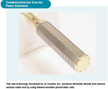
THERMOPHOTOVOLTAIC ELECTRIC POWER GENERATION USING EXHAUST HEAT
Furnaces in the glass, metalcasting, and steel industries operate at very high
temperatures and lose tremendous amounts of energy in their exhaust streams.
With the emissions-reducing shift to gas-oxy furnaces in these industries,
exhaust temperatures are climbing even higher. Waste heat from furnaces in
the glass, metalcasting, and steel industries is usually vented to the atmosphere.
In some facilities, it must be diluted with cool air to reduce its temperature prior
to venting. Until now, the venting of this waste heat has represented the loss of
a valuable resource.
A new technology adds value to this waste stream by using exhaust heat to
generate hundreds of kilowatts of electricity. This unique innovation uses new
infrared-sensitive photovoltaic cells mounted inside ceramic tubes. These tubes
are heated in the exhaust stream of an industrial process and radiate energy
inward to the photovoltaic cells to generate electricity directly from the waste
heat. The energy density in these systems is over 100 times that of solar energy,
producing over 100 times the energy of conventional photovoltaic or solar cells.
Economics and Commercial Potential
Exhaust heat offers an attractive energy alternative to the glass, metalcasting, and steel
industries. In particular, JX Crystals, Inc., has targeted the glass industry because of
an estimated 67 MW of year-round electrical generation available in this industry alone.
The technology has already attracted the partnership of a major glass-industry player
interested in demonstrating the technology on a glass furnace.
Given additional investment in the business and a market volume well over 10 MW per
year, JX Crystals, Inc., estimates the thermophotovoltaic circuit to cost approximately
$0.20 per watt. Balance of system costs are estimated to be $0.50 per watt. Assuming
a price of $1 per watt, utility rates of $0.05 per kWh, and a duty cycle of 90%, the
payback period should be less than 3 years.
This technology could save 27 billion Btu of electricity per installed unit each year. First
sales for the technology are expected by 2004. Based on 25% market penetration by
2010, annual savings could be 0.5 trillion Btu with 18 units installed, each containing 200
5-kW tubes. Market penetration of 50% by 2020 could save 1.0 trillion Btu from the
operation of 37 units by the glass industry.
Subscribe to:
Posts (Atom)

